6.12 EMP_network_analysis

The EMP_multi_analysis module aims to construct network relationships between features to analyze their interactions and identify key feature nodes. This module not only assesses the relationships within single-omics features but also further explores the network interactions between different omics, offering a more comprehensive systems biology perspective.

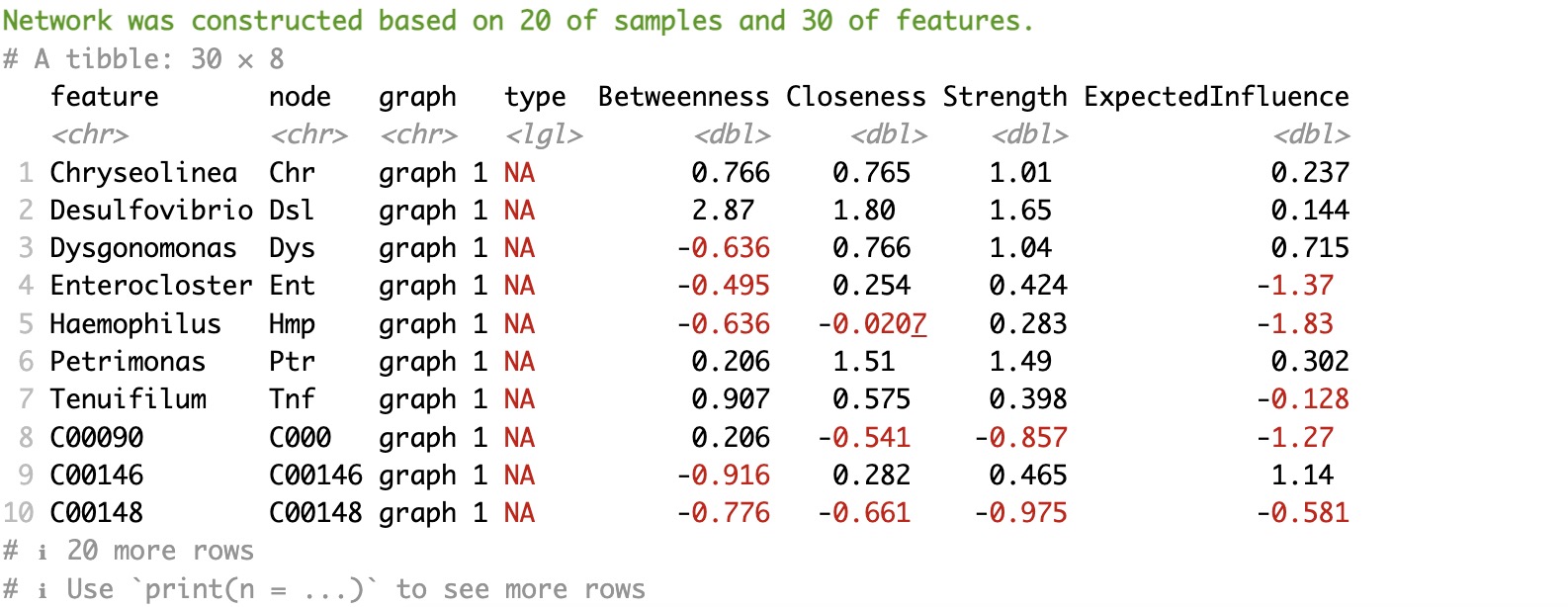
6.12.1 single-omics network

🏷️Example：

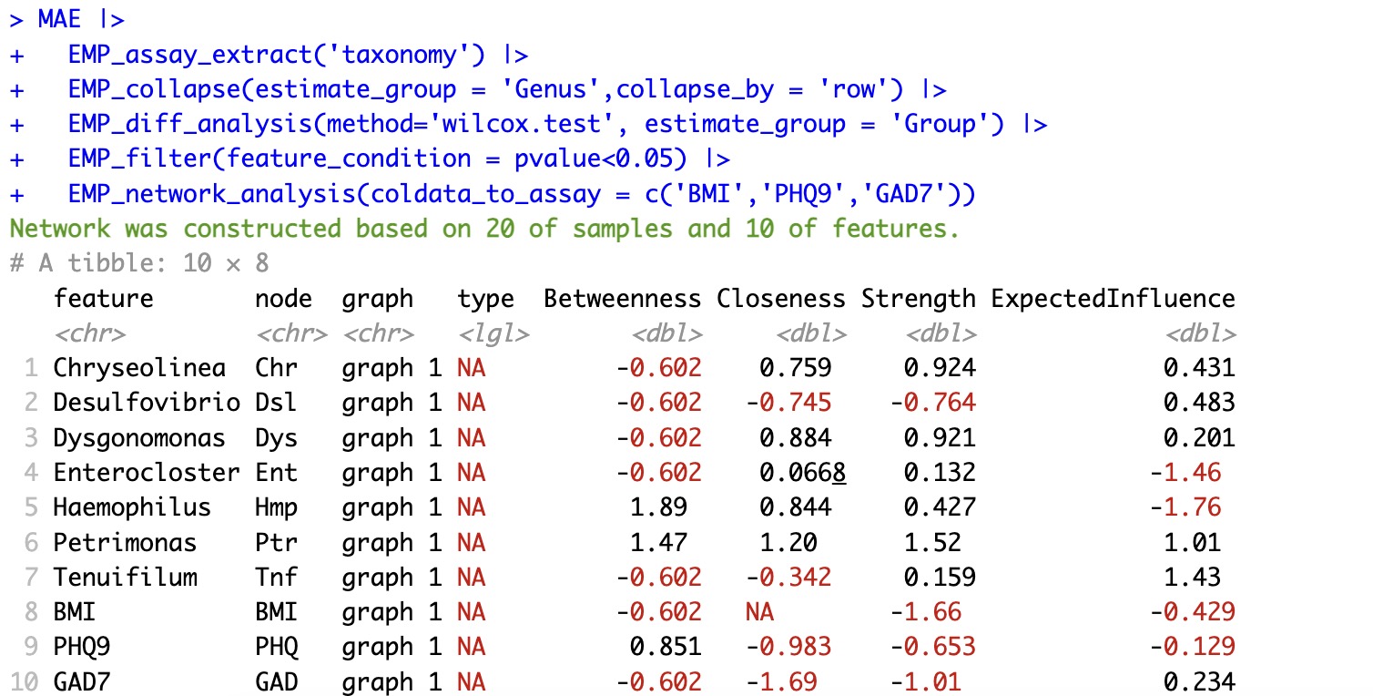
1.Network between differential genus taxa and coldata

Note：
Parametercoldata_to_assaycould inlcude the interesting coldata into the network.

MAE |>
  EMP_assay_extract('taxonomy') |>
  EMP_collapse(estimate_group = 'Genus',collapse_by = 'row') |>
  EMP_diff_analysis(method='wilcox.test、', estimate_group = 'Group') |>
  EMP_filter(feature_condition = pvalue<0.05) |>
  EMP_network_analysis(coldata_to_assay = c('BMI','PHQ9','GAD7'))

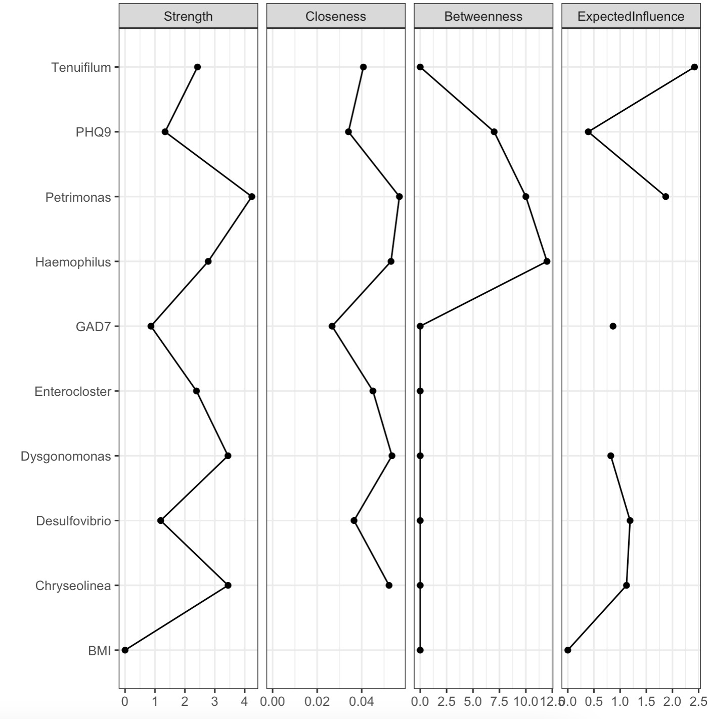
2.Visualization of the node importance.

MAE |>
  EMP_assay_extract('taxonomy') |>
  EMP_collapse(estimate_group = 'Genus',collapse_by = 'row') |>
  EMP_diff_analysis(method='wilcox.test', estimate_group = 'Group') |>
  EMP_filter(feature_condition = pvalue<0.05) |>
  EMP_network_analysis(coldata_to_assay = c('BMI','PHQ9','GAD7')) |>
  EMP_network_plot(show='node')

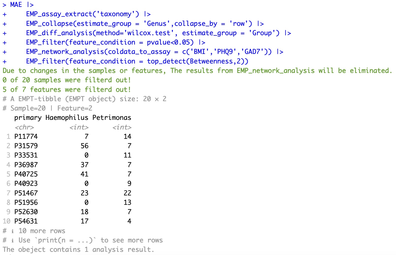
3.Filter the two most important taxa according to the network result

MAE |>
  EMP_assay_extract('taxonomy') |>
  EMP_collapse(estimate_group = 'Genus',collapse_by = 'row') |>
  EMP_diff_analysis(method='wilcox.test', estimate_group = 'Group') |>
  EMP_filter(feature_condition = pvalue<0.05) |>
  EMP_network_analysis(coldata_to_assay = c('BMI','PHQ9','GAD7')) |>
  EMP_filter(feature_condition = top_detect(Betweenness,2))

6.12.2 Multi-omics network

🏷️Example：

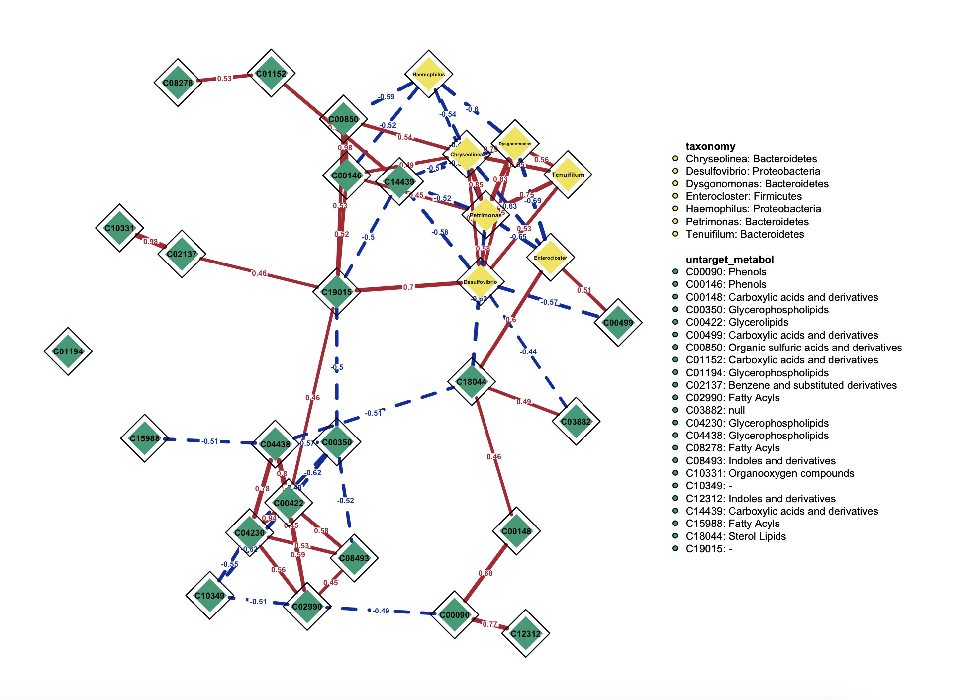
1.Network between microbiome and metabolite

Note：
The parameter threshold can be used to select edges that are statistically significant or edges with adjusted p-values. (Default: threshold='sig')

k1 <- MAE |>
  EMP_assay_extract('taxonomy') |>
  EMP_collapse(estimate_group = 'Genus',collapse_by = 'row') |>
  EMP_diff_analysis(method='wilcox.test', estimate_group = 'Group') |>
  EMP_filter(feature_condition = pvalue<0.05)

k2 <- MAE |>
  EMP_collapse(experiment = 'untarget_metabol',na_string=c('NA','null','','-'),
               estimate_group = 'MS2kegg',method = 'sum',collapse_by = 'row') |>
  EMP_diff_analysis(method='DESeq2', .formula = ~Group) |>
  EMP_filter(feature_condition = pvalue<0.05)

(k1 + k2 ) |> 
  EMP_network_analysis(threshold='sig')

2.Network visualization

Note：
①Paramternode_info could add more info to the node according to their rowdata.
②The parameter threshold here, unlike the one in EMP_network_analysis, specifies the minimum absolute value of the coefficient for edges to be displayed.
③More paramters in the function qgraph.

(k1 + k2 ) |> 
  EMP_network_analysis() |> 
  EMP_network_plot(show = 'net',layout = 'spring',
                   shape='diamond',
                   edge.labels=TRUE,edge.label.cex=0.4,
                   vsize = 5,threshold = 0,
                   node_info = c('Phylum','MS2class'),
                   legend.cex=0.3,label.cex = 1,label.prop = 0.9,font=2)

6.12 EMP_nework_analysis

6.12 EMP_network_analysis

6.12.1 single-omics network

6.12.2 Multi-omics network

results matching ""

No results matching ""